A shopper uploads one photo. Ten seconds later, they’re looking at themselves wearing a garment from a brand's catalog, rendered photorealistically rather than approximated on an avatar. That’s the product. Most of the difficulty sits underneath it.
A single inference pass must resolve pose transfer, cloth deformation, identity, and texture fidelity simultaneously, against a reviewer who can spot an incorrect result instantly but cannot say why. This post covers how the model is built and trained, what the infrastructure had to look like to support it, and a recent inference optimization that reduced per-request latency by 1.7x and more than halved peak memory usage.

Figure 1: Same person, same room, same light. Only the garment is generated.
What the model has to get right
The mental model most people bring to virtual try-on is Photoshop: cut out a garment, warp it onto a photo. That framing breaks immediately, because a garment has no appearance independent of the body wearing it. It has an appearance under a pose, a lighting setup, and a set of material properties. All three have to be inferred from the inputs.
Four problems have to be solved on every inference.
Pose transfer
Catalog photography is controlled. Fixed lighting, deliberate poses, professional models. Consumer photos are whatever the consumer has available: a train platform, a kitchen, a bathroom mirror. The pose, camera angle, and background all differ from the catalog source.
Transferring a garment between those two requires reasoning about the three-dimensional structure of both the source and target poses, and then synthesizing how the garment would fall given the structural differences. A 2D warp cannot do this. It has no way to represent the fact that a sleeve occluded in the source is visible in the target.
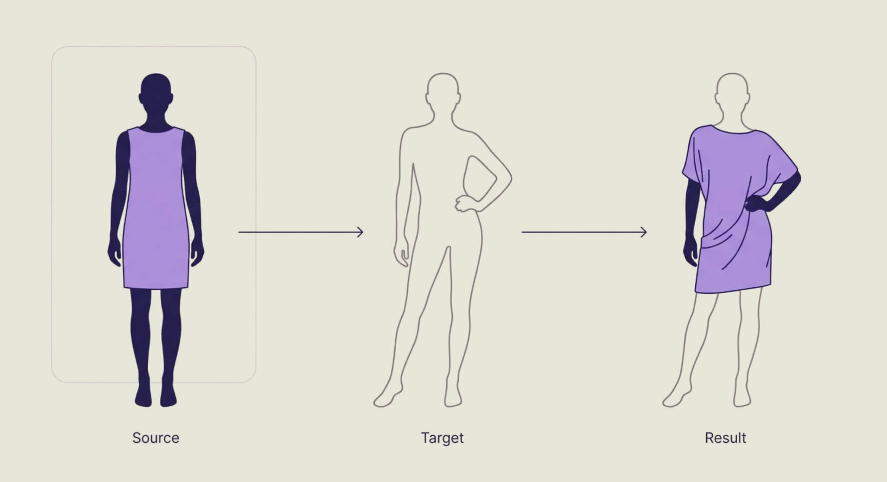 Figure 2: The garment is photographed in one pose and has to appear in another. What changes between source and result is drape, not position.
Cloth deformation
Fabric is not rigid, and every material deforms differently under gravity, tension, and body geometry. Silk drapes where denim holds a crease. A knit bunches at the cuff in a way a woven shirt does not. Sleeves ride up. Collars fold and stay folded.
The model learns this as behavior rather than as an explicit physics simulation, and is trained on large volumes of paired catalog and worn-garment data. The target is not how a garment looks laid flat but how it looks after a body has been inside it for an hour.
Identity
This constraint makes the problem hard rather than merely difficult, and it remains one of the field's more stubborn open problems.
A diffusion model applying a garment to a photo will drift the face. Nose geometry shifts a little. The jawline softens. Skin tone moves half a step. None of it is dramatic, and all of it is noticeable, because the person looking at the output has spent their entire life looking at that face. Drift destroys trust faster than any other failure mode.
SPREEAI treats identity consistency as a hard constraint rather than a loss term to be balanced against others. Dedicated identity-preservation stages sit in the training pipeline, and every checkpoint is validated on embedding similarity against a control set before it can advance. The threshold is high, and the check runs at every critical checkpoint, including when the model reconstructs regions occluded in the source photo.
Texture and logo fidelity
Reviewers do not report that the texture entropy is off. They say the logo looks melted.
"The human eye will pick up very quickly the uncanniness of it. They'll say, 'The logo looks distorted' or 'It's supposed to be an N. Why does it have a carrot on top?'" — Mrinal Shukla, Head of Engineering, SPREEAI
Brand-critical elements have to survive every transformation the model applies. Logos, text, tonal patterns, embroidery. A printed graphic is the hardest case in the set, because it has to deform with the cloth, wrap around the body, and get partially occluded by wrinkles in a physically plausible way, while still reading as the brand's mark rather than a smear.
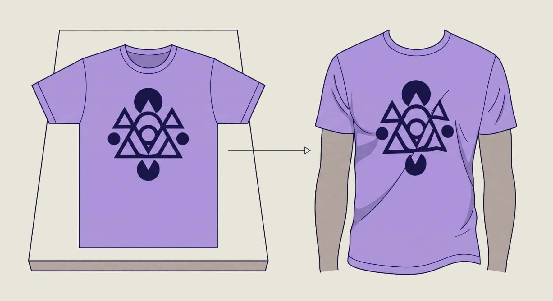
Figure 3: A printed graphic flat-lay (left) has to deform with the cloth and survive the fold (right). Legibility through deformation is the hard part.
From four modules to one model
The first architecture was modular. Separate models for pose estimation, garment segmentation, texture transfer, and identity verification, each feeding the next.
That decomposition matches how the problem is described, which is exactly why it is tempting. It also fails in a specific way: error cascades. A slightly off pose estimate doesn't stay slightly off. It propagates into segmentation, then into texture transfer, and the compounding is not linear. Debugging becomes archaeology, because a visible artifact in the output may originate three stages upstream. Maintaining several models in parallel also splits the team's attention and slows the iteration loop.
SPREEAI is consolidated into a single unified diffusion model that learns the joint distribution across all four problems rather than solving them in sequence. There are no discrete handoffs, so nothing can cascade errors. The model resolves the four constraints against one another and produces a globally consistent result.
The cost of that decision is memory. Holding the joint representation in VRAM during training requires the full 80 GB of an NVIDIA H100 GPU. Memory capacity drove our choice of training hardware, not raw throughput.
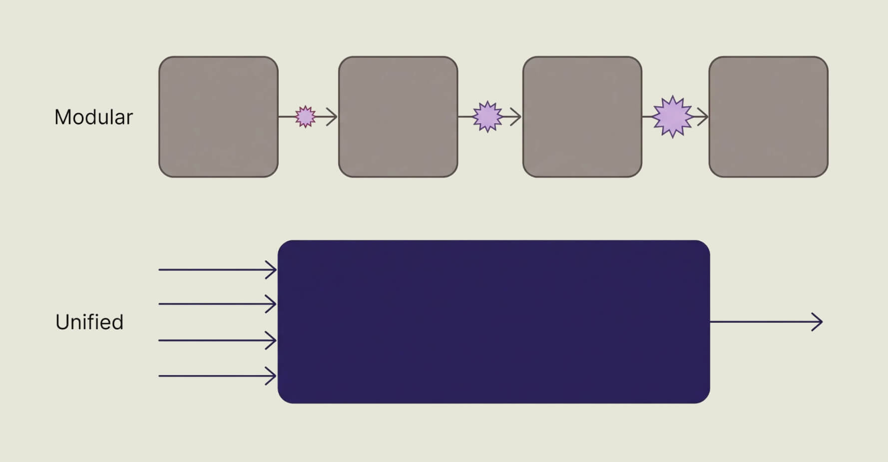
Figure 4: An early error in the chain (top) becomes an input to everything downstream. The unified model (bottom) removes the handoffs that error travels through.
The training pipeline
High-resolution training, quantized inference
Training runs exclusively on high-resolution imagery, because fine detail is exactly what texture and logo fidelity depend on, and it cannot be recovered later if the model never saw it.
Inference runs differently. The model serves in a quantized, lower-resolution mode for speed, and a post-processing stage identifies the regions where fidelity actually matters, meaning text, logos, and faces, then applies targeted upscaling to those regions only. Combined with extra memory allocated to the encode-decode path during inference, this delivers photorealistic output at commercial latency without incurring full-resolution inference end-to-end.
The quantization scheme has since been rebuilt around FP8, for reasons covered in the inference section below.
In short, the original scheme saved memory without adding compute.
Training depth
A full training run reaches up to 50,000 diffusion steps. Each step is a denoising pass in which the model reconstructs a plausible image from noise, conditioned on the garment, the subject's pose, and the target configuration. Fine-tuning passes run 500 to 600 steps with targeted adjustments to specific layers.
This workload doesn't match language model training, and the difference matters for infrastructure. Next-token prediction is comparatively local. Diffusion training requires global consistency across the entire image at every step, with identity, physics, texture, and lighting all coherent at the same time. There is no partial credit for getting the left half of the image right.
Stage ordering
The four problems are interdependent but not equally weighted throughout training, so the pipeline is ordered by dependency:
1. Identity preservation. The foundational constraint everything else has to respect.
2. Texture fidelity. Fine-tuning on high-resolution garment detail, logo, and pattern preservation.
3. Spatial boundary and geometry. Cloth deformation and occlusion handling.
4. Denoising and latent conditioning. Final passes that refine global coherence.
Each stage emits intermediate snapshots, which serve as the regression baseline for the next run. This mechanism drives the compounding growth in data described in the next section. A training iteration does not produce one checkpoint. It produces a checkpoint and the full set of validation artifacts needed to prove that the next iteration is actually better.
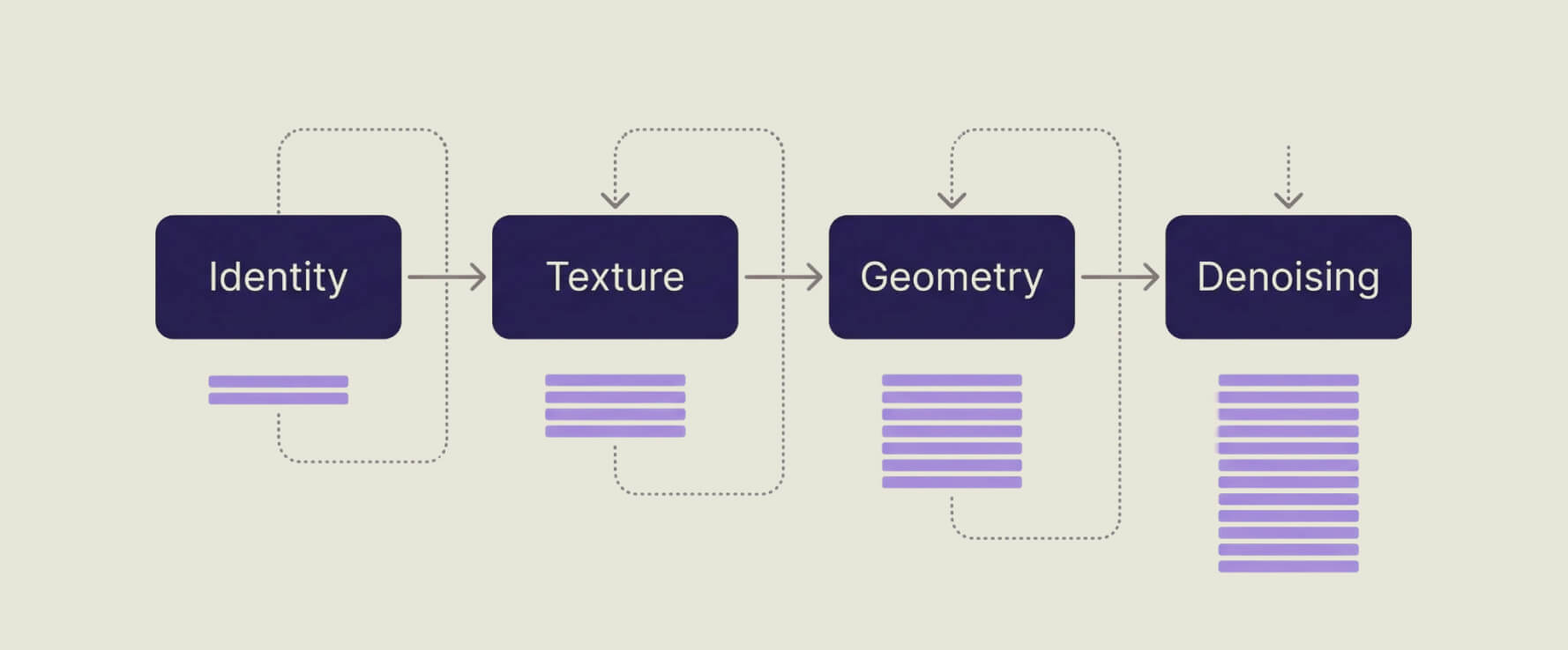
Figure 5: Every stage inherits the artifacts of the stage before it. Storage growth depends on the pipeline shape.
Validation gates
Every critical checkpoint runs parallel validation against a control set:
-
Identity consistency. Embedding similarity between source and output, measured against a fixed threshold.
-
Texture and logo fidelity. Patch-level comparison of brand-critical regions.
-
Cloth physics coherence. Comparison against reference deformation output from the last validated checkpoint.
A checkpoint that misses the threshold does not advance. The gate catches regressions before they propagate into downstream stages, which is the whole point, and it also significantly contributes to artifact volume. Proving a model has not regressed is not free.
Training infrastructure
Why the interconnect matters here
A 50,000-step run takes 7-8 days on an NVIDIA HGX H100 system. At that duration, inter-node communication stops being an implementation detail and becomes a term in the training-time equation.
Distributed data parallelism means every optimizer step requires a full gradient all-reduce across nodes. With a model sized at the limit of NVIDIA H100 VRAM, any delay in gradient exchange lands directly on wall-clock training time, and it compounds across steps.
The communication profile also differs from an LLM in a way that is easy to get wrong when sizing a cluster. LLM attention cost is dominated by a KV cache that grows with sequence length. A diffusion transformer recomputes attention across all spatial tokens at every denoising timestep, so cost scales with step count rather than sequence length. Multiply a small per-step latency by tens of thousands of steps and the fabric becomes the constraint.
Lambda's 1-Click Clusters run a non-blocking NVIDIA Quantum-2 400 Gb/s InfiniBand compute fabric in a rail-optimized topology, delivering up to 3,200 Gb/s of peer-to-peer GPUDirect RDMA between nodes. That kept gradient synchronization off the critical path.
The storage rebuild
By early 2026, the training data estate had grown far past what active work required. The cause was structural, not careless. Every cycle emits checkpoints, latent snapshots, validation outputs, and large volumes of synthetic imagery, and each artifact serves as the regression baseline for the next cycle. Retention was implicit. Nothing had a defined end of life, so nothing ever left.
The rebuild had three parts.
-
Migration under zero egress. Historical training data moved to S3. Lambda charges nothing for ingress, egress, or data transfer, which is what made a bulk migration at that scale something to schedule rather than postpone indefinitely. Egress fees are the reason why many teams keep paying to store data they will never read again.
-
Retention with a defined lifetime. Live storage now holds only what the active run and the current regression baseline require. Everything else moves to S3 immediately after the stage that produced it. Live footprint per cycle dropped by roughly an order of magnitude.
-
Stage-aware sharding. Moving data to S3 traded one bottleneck for another: GPUs began blocking on demand-paged reads. The fix was to shard along the training pipeline's own dependency structure. Identity data, texture data, geometry data, and denoising data are separate shards, pre-staged into Lambda storage before the stage that consumes them runs. The next batch is always local before it is needed, and storage I/O stalls went to zero.
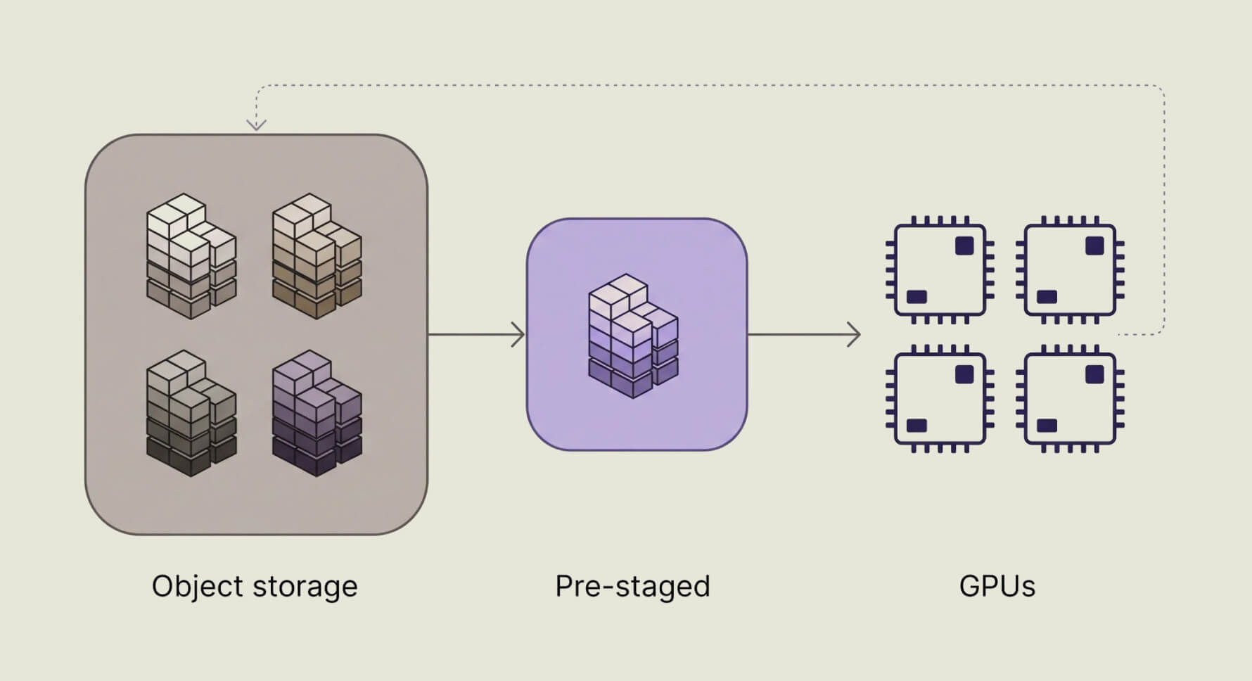
Figure 6: Pre-staging shards for the next batch so data is local before the GPU requests it.
Together, those three changes reduced storage cost by more than 30x.
Fleet occupancy
GPU utilization is two different problems wearing the same name. The first is ensuring reserved GPUs are being fully utilized. The second is how much useful work each GPU accomplishes. They have different causes and different fixes. SPREEAI took them in that order.
At the beginning, a large share of reserved capacity was idle, with utilization averaging in the low 20% even during active training windows. Three causes:
-
Workload fragmentation. Different training features had different memory profiles, but everything landed on NVIDIA H100 GPUs regardless, because the unified model set a memory ceiling for full runs even when only a subset of the model was the training target.
-
No scheduling layer. Jobs were submitted ad hoc, with no priority or queue, which produced contention during some windows and idle reservations during others.
-
Storage I/O blocking. Pre-staging did not exist yet, so GPUs had to wait on reads.
Working with Lambda's ML engineering team, SPREEAI built MLflow-based experiment orchestration on Lambda's stack. Lambda supplied documentation and direct guidance on integration, S3 data pipelines, and GPU observability, and SPREEAI wired Lambda's Prometheus metrics APIs into its own Grafana dashboards.
Three things changed. A structured queue replaced ad hoc submission, so jobs could be matched to GPUs based on actual memory and compute requirements rather than by whoever submitted first. Routing became aware of idle status and workload profile, which cut both contention and over-provisioning. Real-time metrics also made utilization gaps visible that had previously been inferable only after the fact.
Utilization moved from roughly 20% to 43%, against an internal target of 65%. Queue starvation, meaning experiments blocked waiting on an allocation, fell 74% in relative terms.
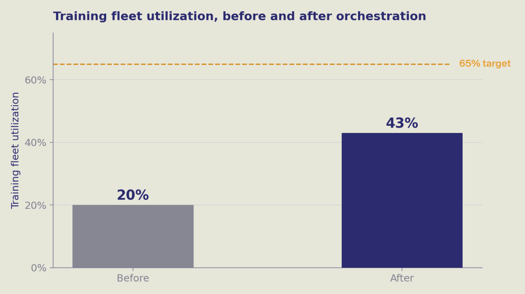
Figure 7: Phase 1—improving GPU utilization with better occupancy via ML orchestration.
That addressed idle capacity. It did nothing about the second problem.
Inference: making each GPU do more
Training runs for weeks. Inference runs in seconds, thousands of times a day, and GPU cost scales directly with customer demand. The second phase of the utilization work targeted the production try-on path itself: a warm, single-request denoising on an NVIDIA H100 GPU with 80 GB of GPU memory, measured end-to-end.
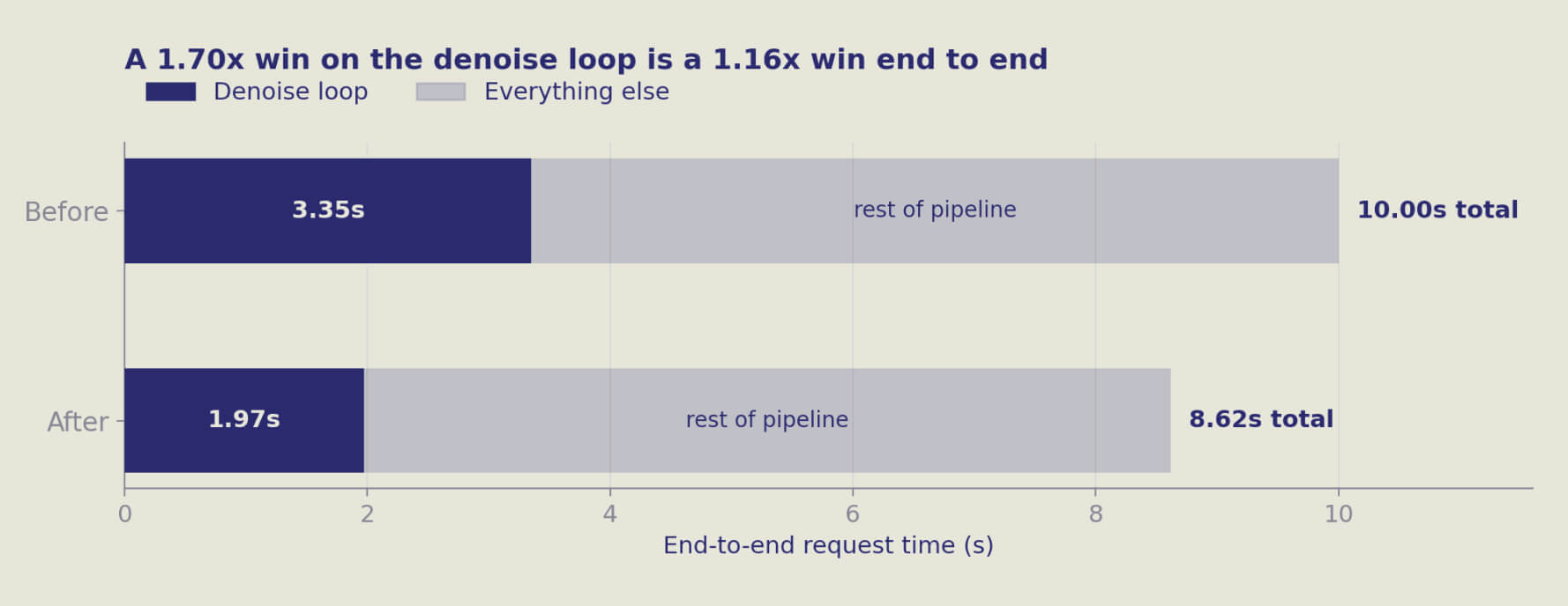
Figure 8: The denoising loop dominates the model call, so optimization targets it exclusively.
The result was a 1.7x per-request speedup with peak GPU memory more than halved, which also increased the number of concurrent try-on requests a single GPU with 80 GB can support from effectively one to somewhere between eight and eleven.
A measuring stick, first
Before any optimization, the team built a fixed benchmark: the exact inputs captured from real try-on requests, a fixed random seed, production math flags, and an already-warm GPU so compile time and preprocessing couldn't contaminate the numbers. Every candidate technique then ran as an isolated experiment against that same stick.
This mattered more than it sounds. An early sweep measured one promising kernel at 2.28s and nearly discarded a better option on that basis. The number turned out to be an artifact of two other GPUs on the same node compiling concurrently, which inflated dispatch time and pushed the node into its power cap. Latency must be measured sequentially on an idle GPU; otherwise you are benchmarking your neighbors.
The finding that reframed the work
The production model already ran int8-quantized weights, which everyone reasonably read as evidence that the model was already optimized. It was not.
The quantization scheme was weight-only. Weights are stored in INT8 to save memory, then dequantized back to BF16 before every matrix multiply. The tensor cores never see an INT8 operand. The model collected the memory savings, but none of the compute savings, which meant a full generation of hardware acceleration was still on the table, hidden behind a label that said the work was done.
Switching the transformer's 109 linear layers to true FP8, where the tensor cores actually execute the low-precision GEMM, delivered 1.24x to 1.28x. Real, and short of the target.
Concurrency, tested and refuted
The obvious way to raise throughput is to run more requests at once, so the team measured it directly rather than assuming.
Two concurrent requests overlapped by less than 7% and under FP8, by around 2%. The model is compute-bound. Every request already saturates the GPU's arithmetic units, so stacking request queues the same work rather than interleaving it.
That is a useful negative result, and it narrowed the search. Concurrency buys density, meaning more requests resident per GPU, but not throughput. The only lever to reduce GPU count is to reduce compute per request.
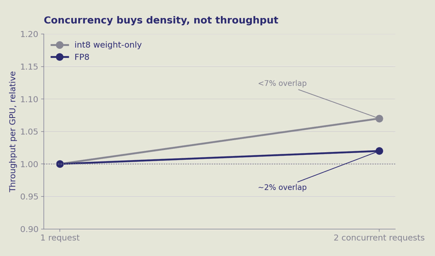
Figure 9: Concurrent requests overlap by less than 7%, and by about 2% under FP8.
Attention was the whole game
A per-kernel profile of the denoising transformer showed attention consuming 54% to 59% of GPU time before FP8 and 73% to 77% after FP8. FP8 shrank only the slice it could reach and left the dominant one untouched.
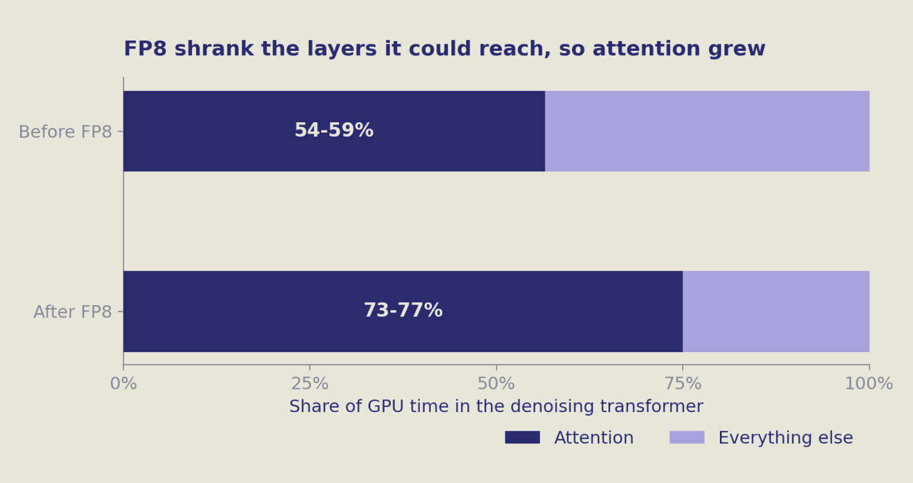
Figure 10: FP8 shrank the linear layers and left attention untouched, resulting in attention growth and higher GPU time.
The fix was a Hopper-specialized NVIDIA cuDNN attention kernel selected in place of the default flash-attention path. It ships with PyTorch, so nothing needed to be built or installed, and the change is a single method call on the model. Production source and configuration are untouched.
How these numbers were measured
Every figure below comes from a single harness: a warm NVIDIA H100 GPU, one request at a time, exact inputs captured from real production try-on requests, a fixed random seed, and production math flags. Runs were timed sequentially on an otherwise idle GPU. Each figure is the median of ten. Latency is denoise-only, which is the portion of the model called the optimization targets. Memory is peak allocation for the request. Concurrency figures are measured at two requests; anything beyond that extends the measured per-request cost and is marked as such.
|
Configuration |
Denoise latency |
Peak GPU memory |
vs production |
|
Production (INT8 weight-only + flash attention) |
2.85 s / 3.35 s |
36.9 / 43.2 GB |
1.00x |
|
FP8 + flash attention |
2.23 s / 2.71 s |
37.0 / 43.4 GB |
1.28x / 1.24x |
|
FP8 + NVIDIA cuDNN attention |
1.66 s / 1.97 s |
17.7 / 19.5 GB |
1.72x / 1.70x |
Two-garment and three-garment requests, respectively. Warm GPU, batch of one, fixed seed.
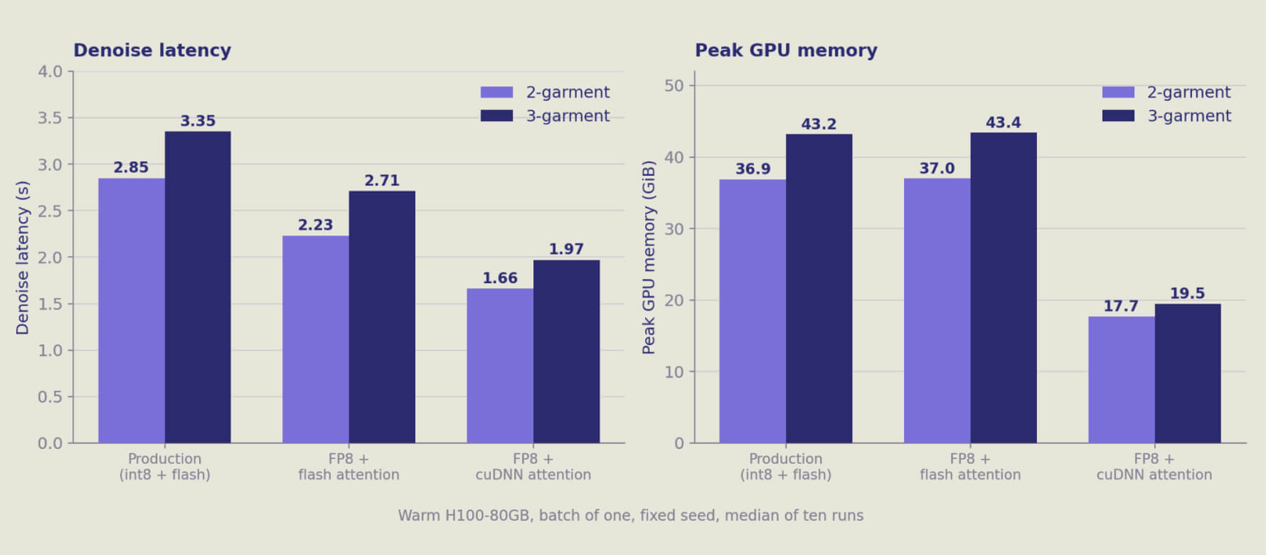
Figure 11: Warm NVIDIA H100 GPU, bs=1. Latency is denoise-only. Memory is peak allocation per request.
Why the memory halved
The memory result was a second-order effect and worth understanding, because it explains where the original spike originated.
The compiler held roughly 35 dequantization intermediates live across the largest graph simultaneously. That was the real source of the peak, a direct consequence of the weight-only quantization scheme. FP8 removes the dequantization step entirely, and the attention kernel swap fragments the remaining graph enough that those buffers are freed as execution proceeds.
Simply integrating the cuDNN kernel into the current INT8 pipeline reduces speed by over 50%, because that workflow relies on compiler fusion, which the new kernel disrupts.
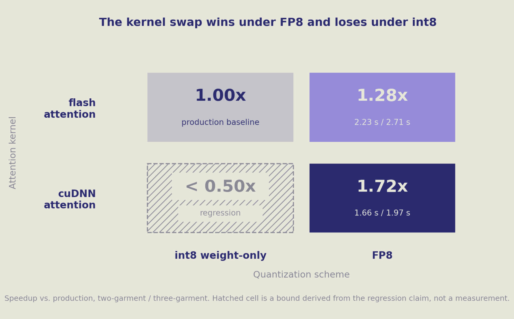
Figure 12: cuDNN attention kernel showed up to 50% regression on INT8 pipeline.
Density, in practice
Under the new stack, a second concurrent request costs only 6-8 GB because the model weights are already resident and only the activations are duplicated. Depending on the garment count, roughly eight to eleven try-on requests now fit on a single NVIDIA H100 GPU: eight for the heavier three-garment shape, and eleven for the two-garment shape.
In the production configuration, two concurrent three-garment requests consumed 74.7 GB, close enough to the 80 GB ceiling that it could not be run safely.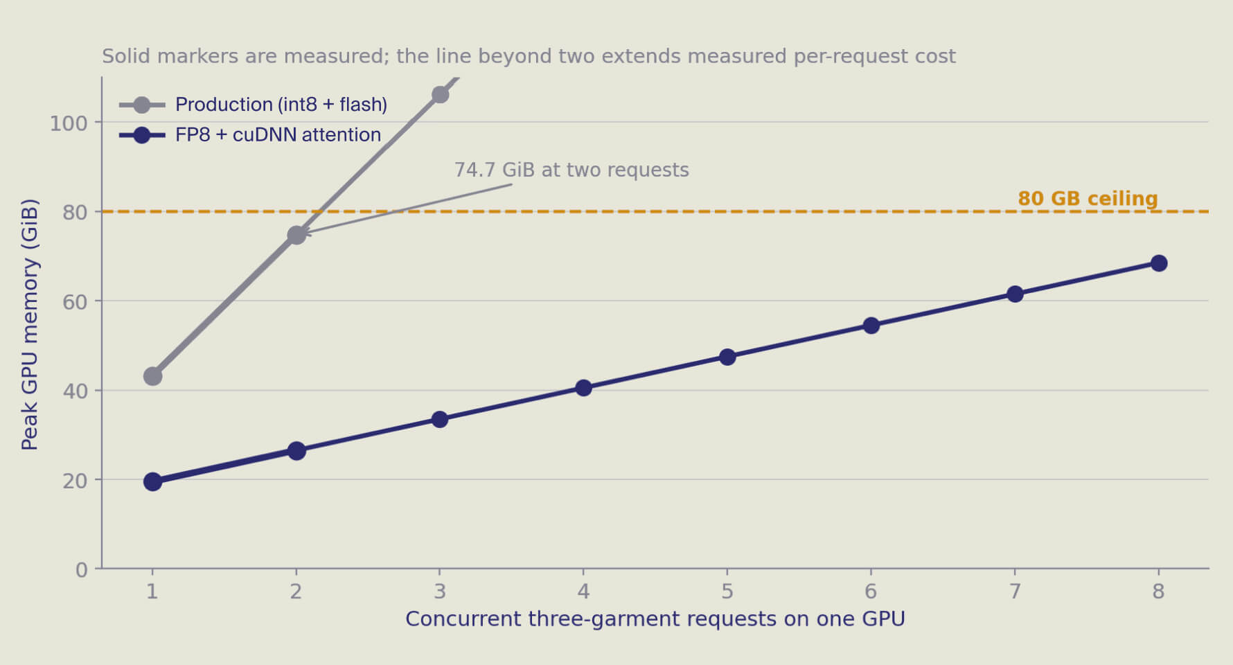 Figure 13: Concurrent three-garment requests on one 80 GB GPU. Solid markers are measured.
The quality question, and why the obvious test is wrong
A faster kernel is only a win if the images are indistinguishable. The instinct is to diff the pixels. For diffusion models, that instinct is wrong, and a control experiment made the point: running the identical attention kernel with and without compilation produced image differences as large as the kernel swap itself.
Diffusion trajectories are chaotic. Any numerical perturbation, anywhere, shifts the path and displaces many pixels without making the image worse. Pixel diff measures trajectory divergence, not quality, and the two are not the same quantity.
So we validated the kernel where the numerics are meaningful: cosine similarity of 0.99998 against the reference attention output, with no numerical instability observed. Final sign-off is a perceptual evaluation on the fine-tuned production weights, the remaining gate before rollout.
"Our goal is not more GPUs, but more efficiency on these GPUs." — Mrinal Shukla, Head of Engineering, SPREEAI
What comes next
Static image try-on is in production. Video is the next frontier, and it introduces temporal consistency as a first-class constraint.
A model can produce a technically correct single frame and still fail on video. Garment position drifts between frames. Physics behaves differently frame to frame. Identity degrades across a sequence. None of these failure modes exist in image generation, and none is addressable by improving single-frame quality, because they are properties of the sequence rather than any frame in it. They require sequence-level training objectives.
The infrastructure implications follow directly. Higher GPU memory per node, higher inter-node bandwidth to move larger gradient tensors from sequence-level objectives, and substantially more data throughput, since video sequences dwarf image pairs.
For that workload, SPREEAI is evaluating NVIDIA GB200 NVL72, which offers 30x real-time throughput over the Hopper generation and a total of 576 TB/s of memory bandwidth. The plan is also to move from data-parallel to tensor-parallel training, distributing the model itself across GPUs rather than only the data. Together with the inference gains above, this is expected to close the gap from 43% toward the 65% target.
Size intelligence is on the near-term roadmap: using the same visual models that already run during try-on to infer fit, predict which size will work for a specific person, and calibrate that prediction to each brand's own sizing conventions. It replaces the size chart and the tape measure with visual inference.
Further out, the platform extends into agentic commerce, with SPREEAI as an embedded intelligence layer serving brands across the supply chain, not just at the point of purchase: procurement, wholesale visualization, and AI-generated catalog content.
"The north star will be a real-time video try-on. You walk into a store, flash a garment on a screen, and see it right on you. We want to be the ones bringing that to the world." — Mrinal Shukla, Head of Engineering, SPREEAI
It all comes back to the same ten seconds. A shopper uploads one photo, and what they get back has to be good enough that they never think about the model, the compute, the kernel, or any of the work described above. They see themselves wearing the thing and decide whether they like it.
Try it at demo.spreeai.com, read the companion case study on the infrastructure work with Lambda, and explore Lambda's 1-Click Clusters.