In Part 1 of this blog post series, I described the preprocessing problem that kept surfacing in conversations with HFT firms: their pipelines are either too rigid or too manual, and neither holds up when market conditions shift. The question I left open was whether there's a more principled alternative, one that doesn't rely on hand-engineering rules for every regime the market might produce.
This post describes what we built to answer that question, what the results showed, and what it means for firms thinking about adaptive risk management.
Key findings
-
A VAE world model produces a genuine regime-instability signal. Trained on 82 days of crypto perpetuals data (BTC, ETH, SOL), the windowed KL surprise signal correlates positively with realized volatility on 77-87% of trading days depending on model variant, with mean flag lift of 4-5× on firing days.
-
The signal leads volatility, not just correlates with it. The standard model leads volatility by a median of +8 events. A predictive variant, trained with a modified objective that orients representations toward future states, achieves up to +90 events of median lead; roughly 9 seconds at 100ms snapshot frequency.
-
The signal adds value over industry-standard baselines. Against rolling realized volatility, the VAE leads by +5 to +91 events depending on model variant. Against Order Flow Imbalance, lead times are comparable, but the VAE produces 36% higher correlation with future volatility, measuring latent market structure rather than instantaneous flow.
-
A systematic grid search mapped the full precision-lead tradeoff. Across 20 model variants (varying regularisation strength β and prediction horizon h), precision clusters tightly between 0.39-0.51 regardless of configuration; precision is structurally bounded. Lead time is the moveable lever, ranging from +8 to +90 events.
-
Three complementary models form a practical alert system. The standard VAE (high precision, short lead), a balanced predictive variant (best day-to-day coverage), and a maximum lead-time variant together provide a three-layer early warning system; 9 seconds, 1.4 seconds, and 0.8 seconds ahead of volatility, respectively.
-
Two honest nulls bound the signal's scope. The per-event KL signal does not flag individual adverse selection at the execution level. The signal is also episodic, silent on 29-40% of days depending on the model, and has not been tested on market stress events beyond the January and March 2024 crypto rally.
The central idea
The core hypothesis is simple: instead of telling the model what normal market behavior looks like, let it learn.
In standard preprocessing pipelines, a human engineer decides how to normalize prices, how to handle volume spikes, which events to filter, and how to treat regime changes. These decisions encode assumptions about the market that may have been valid when the pipeline was written but degrade as conditions evolve. Every time the market enters a new regime, someone has to notice, diagnose, and manually fix the pipeline.
The alternative we explored: train a generative model on historical limit order book data, let it build an internal probabilistic picture of what the market normally looks like, and then use the degree to which new incoming data deviates from that learned picture as a meaningful signal. That deviation, measured as a formal statistical quantity called KL divergence, tells you not just that something has changed, but how much the current state of the market challenges the model's existing understanding.
The key architectural insight, borrowed from reinforcement learning research on intrinsic motivation, is that this signal should be measured against a learned prior rather than a fixed one. A fixed prior (a standard Gaussian distribution) tells you when the data is unusual in an absolute sense. A learned prior, one that has absorbed the structure of the market from historical data, tells you when the data is unusual relative to everything the model already knows. That distinction is what makes the signal meaningful rather than just noisy.
What we built
The world model
We built a sequential β-VAE (Variational Autoencoder) with a GRU-based learned prior. In plain terms: a neural network that reads sequences of limit order book snapshots, compresses them into a compact latent representation, learns to reconstruct them, and simultaneously learns a temporal model of how those representations evolve from one moment to the next.
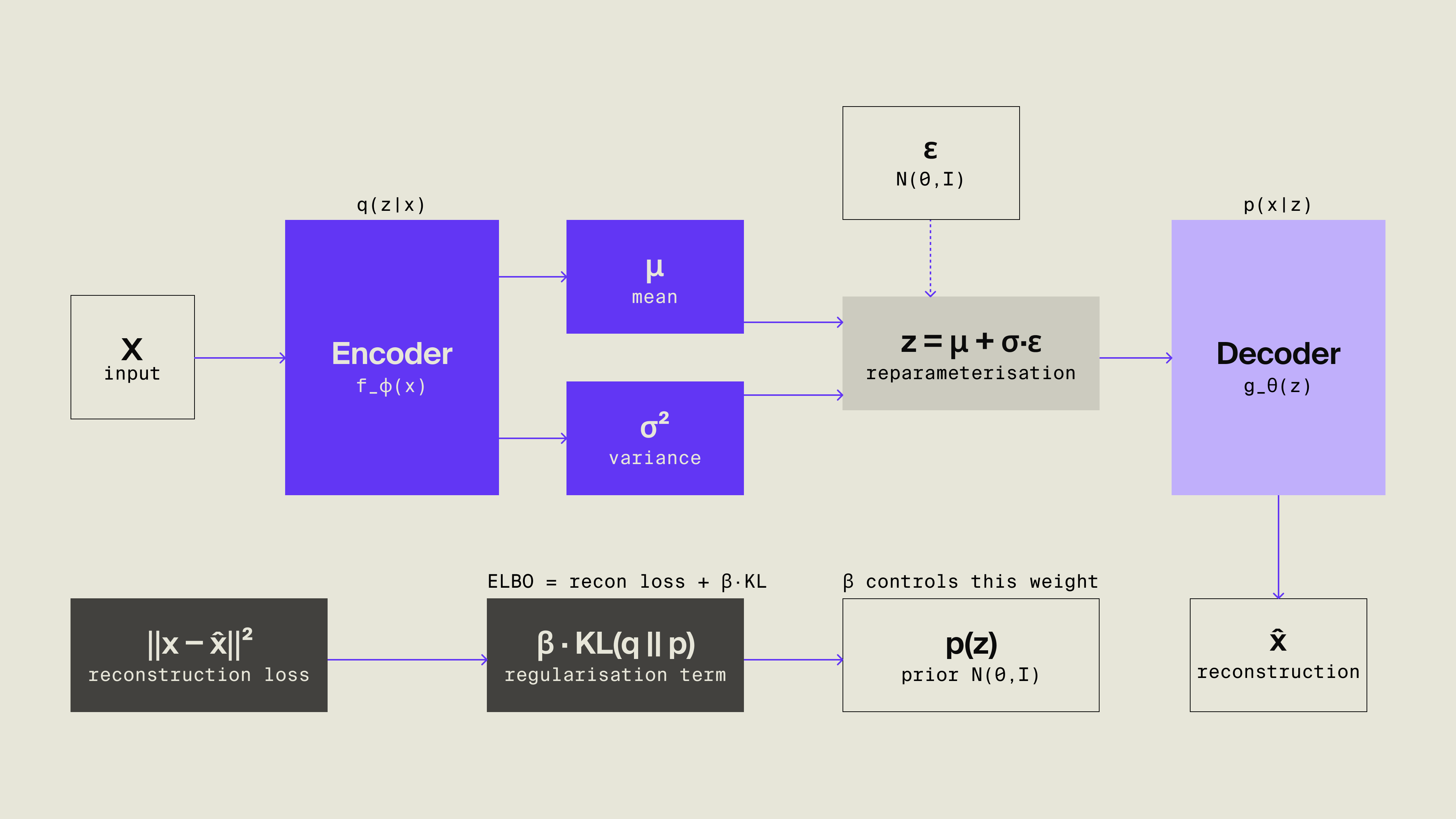
The state representation captures the full microstructure of the order book at each event: five price levels on each side, with prices expressed relative to the mid-price and volumes normalized via causal rolling z-score, plus a one-hot encoding of the event type (submission, cancellation, execution, halt). Each state vector is 47 dimensions; the model processes sequences of 100 consecutive events at a time.
The learned prior is a GRU network that takes the sequence of previous latent states and predicts where the next latent state should be, given everything the model has seen so far. KL divergence between the model's posterior (what it actually encodes from the new observation) and this learned prior (what it expected to see) is the surprise signal.
High KL → the current market state is genuinely unexpected relative to the model's world model.
Low KL → the market is behaving as anticipated.
Training used β-annealing (gradually increasing the weight on the KL term from 0 to β_max over the first half of training) and free bits (a minimum KL floor per latent dimension) to prevent posterior collapse, the failure mode where the model ignores the latent space entirely. All 16 latent dimensions remained active throughout training with zero collapse across all experiments.
Why this is different from existing approaches
Most LOB representation learning work (including the closely related SimLOB, 2024) trains a generative model and uses the learned representations as input features for a downstream prediction task. The representation is learned in service of the task.
What we're doing is different: the KL surprise signal itself is the output, not an intermediate representation. We're not asking "can a VAE help us predict mid-price movement better?" We're asking "can a VAE's measure of surprise tell us something useful about the current state of the market, independent of any specific prediction task?" That reframing opens up a different set of applications (regime detection, risk management, execution quality monitoring) that don't require the signal to be predictive in the traditional sense.
Dataset and methodology
Why crypto perpetuals
We began with LOBSTER equity data (AAPL, AMZN, MSFT, one trading day in 2012) and quickly identified a fundamental limitation: one calm equity day gives the model a single regime to learn from. Its definition of "normal" is essentially "what June 21, 2012 looked like." A surprise signal trained on one regime has limited ability to distinguish genuine novelty from routine variation.
We extended to Binance USD-M futures book depth snapshots (BTC, ETH, and SOL) covering January and March 2024: 82 trading days, approximately 4,340 training sequences. Crypto perpetuals provided exactly what equity data could not: genuine regime diversity across a sustained volatile period. March 2024 saw BTC rally from $50k to $73k, a multi-week trend change with significant intraday volatility spikes across all three assets simultaneously. This is the kind of data a world model needs to learn what "genuinely unusual" looks like.
Data note: Binance bookDepth uses percentage-band snapshots rather than discrete price levels. Per-level price is derived: Δ notional/ Δ depth and volume as Δ depth (de-cumulated). This representation is coarser than exchange-native tick data, a documented limitation.
The validation design
We tested the surprise signal on two distinct questions, chosen because they represent real operational concerns for market makers:
Question 1 (adverse selection): Do individual executions that the VAE finds surprising suffer larger adverse price moves against a passive market maker? This tests whether the per-event KL signal can flag potentially toxic order flow.
Question 2 (regime instability): Does the KL signal, aggregated over rolling windows of 500 events, couple with realized volatility, and does it precede it?
We also benchmarked against two industry-standard signals computed over the same 500-event window: rolling realized volatility and Order Flow Imbalance (OFI).
Results
Question 1: adverse selection, the honest null
The per-event KL signal does not flag adverse selection. Across all three equity tickers, high-KL executions didn't suffer larger adverse price moves than low-KL executions:
| Ticker | hi-KL adverse (cents) | lo-KL adverse (cents) | hi-lo | corr(KL, adverse) |
|---|---|---|---|---|
| AMZN | 1.10 | 1.40 | −0.30 | −0.061 |
| AAPL | 1.52 | 1.57 | −0.05 | −0.008 |
| MSFT | 0.20 | 0.19 | +0.01 | +0.030 |
This is a meaningful negative result. The signal encodes what type of event occurred (executions are consistently more surprising than submissions, KL ratios of 1.17×, 1.40×, and 1.99× for AMZN, AAPL, and MSFT) but not whether a specific execution is informed.
Question 2: regime instability, a positive signal
The windowed KL signal shows genuine, consistent coupling with realized volatility across 155 day/asset combinations:
| Metric | BTC (n=62) | ETH (n=62) | SOL (n=31) | All (n=155) |
|---|---|---|---|---|
| % days corr(KL,vol) > 0 | 71.0% | 77.4% | 90.3% | 77.4% |
| Median corr(KL,vol) | 0.395 | 0.408 | 0.509 | 0.435 |
| % days signal fires (lift > 1) | 33.9% | 43.5% | 51.6% | 41.3% |
| Mean lift when fires | 5.43× | 4.70× | 5.50× | 5.14× |
| Mean precision when fires | 0.543 | 0.470 | 0.550 | 0.514 |
| Median lead (positive days) | +5.5 | +6.0 | +10.0 | +8.0 |
Three findings stand out:
- Coupling strengthens with asset volatility: SOL (most volatile) shows tightest coupling at 90.3% of days positive.
- When the signal fires it fires with high precision: the March 2024 cluster showed 9-10× lift simultaneously across all three assets during the BTC $50k→$73k rally.
- The signal leads volatility by a median of +8 events on positive-corr days: it fires before volatility materialises, not after.
Baseline comparison
To assess whether the signal adds genuine value over what practitioners already compute, we compared against two industry-standard baselines over the same 500-event window:
| Signal | Median lag | Mean corr(future vol) | % days VAE leads more |
|---|---|---|---|
| VAE KL (standard) | +4 events | 0.343 | — |
| Rolling vol (autocorrelation) | −1 events | 0.998* | 72.3% |
| Order flow imbalance (OFI) | +7 events | 0.253 | 45.2% |
- Near-perfect due to overlapping windows, not genuine predictive power
The VAE leads volatility by +5 events over rolling vol on 72.3% of days. Against OFI the lead time is roughly tied, but the VAE produces 36% higher correlation with future volatility (0.343 vs 0.253). The VAE and OFI are measuring fundamentally different things, instantaneous order flow imbalance versus latent market structure, which means they are complementary rather than redundant signals.
Going further: the predictive VAE
The baseline comparison raised an obvious question: if the goal is lead time, can we do better than +4 events?
The standard VAE is trained to reconstruct the current state, encode snapshots 1-100, reconstruct snapshots 1-100. This means the latent representation is optimized to describe what is happening now, which is why the surprise signal fires roughly simultaneously with the onset of volatility.
We made one change to the loss function: instead of comparing the decoder's output against the input it just saw, we compared it against the input shifted forward by h events. The model now encodes snapshots 1-80 and must reconstruct snapshots 21-100.
Standard VAE: encode x[1:100] → reconstruct x[1:100]Predictive VAE: encode x[1:80] → reconstruct x[21:100] (h=20)
This single change, one line of code in the loss function, forces the encoder to learn features that are predictive of the future rather than descriptive of the present. The KL signal then fires when the current state of the market is inconsistent with what the model expects the future to look like, rather than what it expects the present to look like. The result is a naturally forward-looking surprise signal.
We also found that β (the regularisation weight on the KL term) significantly amplifies this effect. Higher β forces the latent space to be more structured, which couples the encoder more tightly to the temporal prediction task and pushes the effective lead time further ahead.
Results across model variants
We ran a systematic grid search across β ∈ {1.0, 1.5, 2.0, 3.0, 4.0} and prediction horizon h ∈ {0, 10, 20, 30, 50}, training 20 models in total. The full sweep revealed a clear Pareto frontier between lead time and signal quality:
| Model | β | h | % days corr>0 | Median corr | % fires | Precision | Median lag |
|---|---|---|---|---|---|---|---|
| Standard | 1.0 | 0 | 77.4% | 0.435 | 41.3% | 51.4% | +8 events |
| Balanced early warning | 2.0 | 10 | 87.1% | 0.445 | 52.3% | 44.1% | +14 events |
| High firing rate | 4.0 | 20 | 80.0% | 0.384 | 56.1% | 44.7% | +21 events |
| Maximum lead time | 2.0 | 50 | 75.5% | 0.238 | 47.7% | 42.6% | +90 events |
The β=2.0, h=50 model achieved +90 events of median lead, roughly 9 seconds at 100ms snapshot frequency. This is the largest lead time of any model tested, by a substantial margin.
The β=2.0, h=10 model emerged as the most reliable day-to-day signal: highest percentage of days with positive correlation (87.1%), highest median correlation (0.445), and a +14 event lead, a strong balanced option when consistent coverage matters more than maximum warning time.
Two structural findings held across all 16 models: precision clusters tightly between 0.39-0.47 regardless of β or h, there appears to be a natural precision ceiling for this signal type, and β interacts with h in a non-monotonic way at long horizons. At h=50, β=2.0 produces +90 events but β=4.0 produces only +42, suggesting that over-regularisation at long horizons degrades rather than amplifies the lead time advantage.
A three-signal system
The grid search revealed that the standard and predictive variants are not competing but complementary, each answering a different question at a different time horizon. The three models that together form the most useful operational system are:
- β=2.0, h=50, maximum lead time alert: fires ~9 seconds before volatility materialises. Lower precision (42.6%) but the earliest possible warning. Fires on 47.7% of days.
- β=2.0, h=10, balanced early warning: fires ~1.4 seconds ahead. The most reliable day-to-day signal, highest % days corr>0 (87.1%) of any model tested. Fires on 52.3% of days.
- Standard VAE (β=1.0, h=0), high precision confirmation: fires ~0.8 seconds ahead. Highest precision (51.4%). The signal to act on aggressively. Fires on 41.3% of days.
Deployed as a three-layer alert system:
| State | Action |
|---|---|
| All signals silent | Trade normally |
| 9-second alert only | Pre-position, monitor closely |
| 9-second + 1.4-second alert | Widen spreads, reduce quote size |
| All three fire | Aggressive spread widening, reduce inventory |
| Confirmation only (early warnings missed) | Act immediately, signal arrived late |
This structure mirrors how experienced risk managers already think: a distant, uncertain signal prompts vigilance; a closer, more reliable signal prompts preparation; a high-confidence confirming signal prompts action. The three-layer system provides all three, derived from a single underlying world model trained once on historical data.
Honest limitations
The signal is episodic. It fires on 41-53% of days depending on model variant and is completely silent on 31-38%. It is not a continuous risk meter.
Precision is moderate. 43-51% precision when firing is meaningfully above base rate but leaves substantial room for false alarms. A market maker using this signal will widen spreads on days when volatility does not materialise.
Single volatile period tested. All results come from January and March 2024. Whether the signal generalises to flash crashes, liquidity crises, or macro shocks is untested.
No adverse selection at the individual order level. The per-event signal does not flag individual toxic executions, only aggregate regime-level instability.
Snapshot data approximation. Binance bookDepth is coarser than exchange-native tick data. Results on true L2 order book data may differ.
What we would do next
Speculative decoding-inspired hybrid. The two-signal system currently runs both models independently. A more tightly coupled architecture would feed the predictive VAE's forecast latents as additional conditioning to the standard VAE's prior, analogous to how speculative decoding in LLMs feeds a draft model's proposed tokens to a verifier. The standard VAE's KL signal would then measure surprise given both recent history and the predictive model's forecast, potentially recovering precision without sacrificing lead time.
Market-making simulation. With the regime signal validated as a leading indicator, the natural next step is a market-making simulation that acts on it, widening spreads when KL is elevated, and tests whether this produces better outcomes than a fixed-spread strategy.
More stress regimes. Extending to the 2022 crypto crash, exchange outages, and macro events would test whether the regime-coupling finding is stable across different types of market stress.
Ensemble disagreement. Training multiple VAEs and using disagreement rather than raw KL as the surprise signal would improve separation between genuine epistemic novelty and irreducible market noise.
Closing note
The most important methodological point in this work is the sequence of honest tests. We started with a hypothesis (KL surprise helps a trading agent), found a correct null, reframed (is the signal descriptive of regime structure?), found a partial positive, pushed further (does it lead volatility?), found a clear positive, benchmarked against industry signals, extended to a predictive variant, and swept hyperparameters to map the precision-lead tradeoff.
That sequence matters. A signal that has been tested against nulls and found to fail in one application is more credible when it succeeds in another. The regime-instability finding is stronger precisely because we know what the signal cannot do.
To see the code and experiment outputs, talk to our team.
Appendix A
Full grid search results
Complete results across β ∈ {1.5, 2.0, 3.0, 4.0} and prediction horizon h ∈ {10, 20, 30, 50}, 16 models total. All models trained on the same Binance BTC/ETH/SOL dataset (Jan–Mar 2024, 155 day/asset combinations). Regime detector run with a rolling window of 500 events, max lag ±200 events.
| β | h | % days corr>0 | Med corr | % fires | Lift | Precision | Med lag | % silent |
|---|---|---|---|---|---|---|---|---|
| 1.5 | 10 | 81.3% | 0.399 | 49.0% | 4.54× | 0.454 | +9 | 32.3% |
| 1.5 | 20 | 81.9% | 0.352 | 48.4% | 4.67× | 0.467 | +21 | 34.2% |
| 1.5 | 30 | 73.5% | 0.271 | 45.2% | 4.36× | 0.436 | +37 | 35.5% |
| 1.5 | 50 | 75.5% | 0.260 | 49.7% | 4.29× | 0.429 | +47 | 29.7% |
| 2.0 | 10 | 87.1% | 0.445 | 52.3% | 4.41× | 0.441 | +14 | 31.6% |
| 2.0 | 20 | 81.9% | 0.327 | 52.9% | 4.33× | 0.433 | +38 | 31.0% |
| 2.0 | 30 | 74.8% | 0.336 | 49.0% | 4.40× | 0.440 | +33 | 32.9% |
| 2.0 | 50 | 75.5% | 0.238 | 47.7% | 4.26× | 0.426 | +90 | 34.2% |
| 3.0 | 10 | 83.2% | 0.364 | 47.1% | 4.54× | 0.454 | +15 | 36.1% |
| 3.0 | 20 | 82.6% | 0.352 | 51.6% | 4.73× | 0.473 | +19 | 30.3% |
| 3.0 | 30 | 70.3% | 0.215 | 43.2% | 3.96× | 0.396 | +51 | 40.0% |
| 3.0 | 50 | 73.5% | 0.241 | 51.6% | 4.35× | 0.435 | +34 | 28.4% |
| 4.0 | 10 | 85.2% | 0.358 | 54.2% | 4.71× | 0.471 | +23 | 30.3% |
| 4.0 | 20 | 80.0% | 0.384 | 56.1% | 4.47× | 0.447 | +21 | 29.7% |
| 4.0 | 30 | 77.4% | 0.299 | 45.2% | 4.74× | 0.474 | +28 | 38.7% |
| 4.0 | 50 | 67.1% | 0.239 | 51.0% | 4.21× | 0.422 | +42 | 32.9% |
Column definitions:
- % days corr>0, percentage of 155 days where windowed KL positively correlates with realized volatility
- Med corr, median Spearman correlation between windowed KL and windowed realized volatility across all days
- % fires, percentage of days where windowed KL enters its top decile (flag lift > 1×)
- Lift, mean flag lift on firing days (how many times more likely is a high-vol window when KL is elevated vs base rate)
- Precision, mean precision on firing days (fraction of top-decile KL windows that coincide with high-vol windows)
- Med lag, median lead time in events on positive-corr days (positive = KL leads volatility)
- % silent, percentage of days where top-decile KL never coincided with a high-vol window
Notable observations:
- Precision is structurally bounded at 0.39–0.47 across all 16 combinations; lead time is the moveable lever, not precision
- β=3.0, h=30 is a local minimum, lowest lift (3.96×), lowest corr (0.215), highest silent rate (40%)
- β effect is non-monotonic at long horizons: at h=50, β=2.0 produces +90 events but β=4.0 produces only +42
- All models showed zero posterior collapse and full latent dimension utilization throughout training
References
¹ Wu Y, Mahfouz M, Magazzeni D, Veloso M. Towards robust representations of limit order books for deep learning models. arXiv. 2021. arXiv:2110.05479.
² Zhong M, Lin Y, Yang P. Representation learning of limit order book: a comprehensive study and benchmarking. arXiv. 2025. arXiv:2505.02139.
³ Li Z, Liu W, Bian J, et al. SimLOB: learning representations of limited order book for financial market simulation. arXiv. 2024. arXiv:2406.19396.
⁴ Kingma DP, Welling M. Auto-encoding variational Bayes. arXiv. 2013. arXiv:1312.6114.
⁵ Higgins I, et al. beta-VAE: learning basic visual concepts with a constrained variational framework. ICLR. 2017.